

If I had to track solar performance with one checklist, I’d use six KPI groups: production, availability, service tickets, labor use, project margin, and billing speed.
Here’s the short version: SCADA tells me what the plant did. ERP tells me what that did to costs, labor, revenue, and cash. When I connect those two, I can spot output loss, service delays, margin drift, and slow invoicing before they pile up.
At a glance, I’d watch:
- Production: total generation, specific yield, PR, temperature-corrected PR, capacity factor, EPI
- Uptime: technical, contractual, and energy-based availability, plus MTTR and MTBF
- Service: response time, resolution time, ticket age, closure rate, repeat failure rate, first-time fix rate
- Labor: technician utilization, labor cost per work order, repeat visits
- Margin: gross margin %, budget vs. actual margin, cost per watt, O&M cost per MWh, rework cost
- Cash flow: days to invoice, unbilled completed work, DSO, AR aging, collection rate
A few numbers stand out right away:
- Capacity factor: often 20%–30% for U.S. utility-scale PV
- EPI: many contracts look for 0.95–1.05
- MTTR for critical inverters: often under 4 hours
- Technician utilization: often 65%–80%
- Preventive work: often 60%–70% of total tickets
- Days to invoice: 0–14 days is a strong target
- Contractual availability: often 98%+, based on the contract
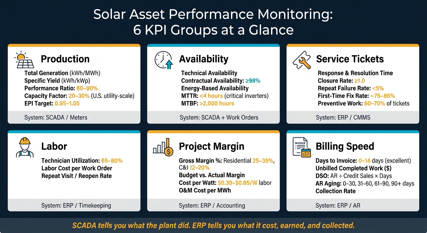
Quick Comparison
| KPI Group | What I’m checking | Main system |
|---|---|---|
| Production | Output vs. model | SCADA / meters |
| Availability | Downtime and lost energy | SCADA + work orders |
| Service | How fast issues are handled | ERP / CMMS |
| Labor | Time use and crew cost | ERP / timekeeping |
| Margin | Profit by job or service work | ERP / accounting |
| Billing | How fast work turns into cash | ERP / AR |
Bottom line: I’d build one monthly scorecard with clear owners, fixed review dates, and action limits, so every drop in kWh, every open ticket, and every delayed invoice has a next step.
Production and Availability KPIs
Production KPIs to Track at Every Site
Six core production KPIs show how a solar asset is performing against design expectations.
Total generation is the baseline. It’s measured in kWh for smaller commercial sites and in MWh or GWh for utility-scale plants. Most teams pull it from revenue meters or SCADA in 5- to 15-minute intervals, then roll it up into daily, monthly, and annual totals.
Specific yield (kWh/kWp) puts output in relation to DC nameplate capacity, which makes it easier to compare sites of different sizes. If yield comes in 5% to 10% below the model, that’s a sign to check for soiling, shading, or inverter trouble.
Performance Ratio (PR) shows how well the system turns irradiance into AC energy under IEC 61724. In hot climates, use temperature-corrected PR so you can separate weather from equipment loss.
Capacity factor compares actual output with what the plant would have produced if it ran at full capacity for the same time period. U.S. utility-scale PV plants usually land in the 20% to 30% range.
The Energy Performance Index (EPI) compares actual production to modeled expected production. This one matters for contract risk. Many lender covenants and PPA agreements look for EPI between 0.95 and 1.05. If it stays below 0.95, that can lead to financial fallout, including liquidated damages or lower distributions.[5]
Store modeled production baselines in ERP by site. Then, when meter data comes in through API or batch import, compare actual output, revenue, and contract performance against budget.
Once you’ve benchmarked output, availability metrics help explain where any gap is coming from.
Downtime and Availability KPIs
Track three types of availability: technical availability, contractual availability, and energy-based availability.
- Technical availability leaves out planned downtime and grid outages outside your control.
- Contractual availability follows the exclusion rules written into the O&M agreement or PPA.
- Energy-based availability weighs downtime based on lost output.[5][6][7]
Use MTTR to measure average repair time and MTBF to measure operating time between failures. A solid starting point is MTTR under 4 hours and MTBF above 2,000 hours for critical inverters.[10]
Each downtime event should link back to an ERP work order. That record should include labor hours, parts, repair cost, lost generation, and lost revenue.
Operations Review KPI Table
Use the table below to standardize review by owner, cadence, and ERP field.
| KPI | Formula | Unit | Typical Target | Primary System of Record | ERP Financial Field |
|---|---|---|---|---|---|
| Total Generation | Sum of AC energy over period | kWh / MWh | Per modeled design | Revenue Meter / SCADA | Actual vs. budgeted revenue |
| Specific Yield | Total kWh ÷ DC nameplate (kWp) | kWh/kWp | 1,100–1,800 (region-dependent) | SCADA | Asset/portfolio benchmarking |
| Performance Ratio (PR) | AC energy ÷ (DC capacity × POA irradiance) | % | 80–90% | SCADA + irradiance sensor | Revenue variance |
| Temp-Corrected PR | PR adjusted for module temperature | % | Should align with standard PR target | SCADA + temp sensor | Weather-adjusted variance |
| Capacity Factor | AC energy ÷ (AC nameplate × period hours) | % | 20–30% (U.S. utility-scale) | SCADA / Meter | Modeled vs. actual output |
| Energy Performance Index (EPI) | Actual generation ÷ modeled generation | Ratio | 0.95–1.05 | SCADA + energy model | Contract compliance, penalties |
| Technical Availability | (Total time – fault time) ÷ total time | % | Site-specific | SCADA alarms / ERP work orders | Lost generation (MWh, $) |
| Contractual Availability | Time-based, per contract exclusion rules | % | ≥98% (contract-defined) | SCADA + ERP | PPA penalty / bonus tracking |
| Energy-Based Availability | Actual energy ÷ (actual + lost energy) | % | Site-specific | SCADA + energy model | Lost revenue per incident ($) |
| MTTR | Total repair time ÷ number of repairs | Hours | <4 hours for critical inverters; site-specific by component | ERP work orders | Labor + parts cost per event |
| MTBF | Total uptime between failures ÷ failure count | Hours | >2,000 hours (critical components) | ERP / CMMS maintenance logs | Spare-parts planning, warranty risk |
Service Tickets and Labor Utilization KPIs
Service Ticket KPIs That Show Response Quality
Production KPIs show what a site produced. Service ticket KPIs show how your team reacted when something broke.
That difference matters.
If production drops, ticket data helps you see why. You can trace an outage from the first alarm to the repair, then from the repair to the final cost. Put those two views together, and availability gaps start to make sense.
Track acknowledgment, intervention, response, and resolution as separate timestamps. Use response time for SLA reporting and resolution time for the verified fix.[5]
Those core timestamps are only part of the story. You should also track open tickets by age, backlog by priority, and closure rate.
- Open-ticket age shows where work is getting stuck
- Backlog by priority shows whether high-priority issues are piling up
- Closure rate shows whether your team is closing work faster than new work is coming in
A closure rate below 1.0 means backlog is growing. If ticket age is rising while closure rate is falling, that’s usually a staffing or dispatch issue.
Two more KPIs help round out response quality: repeat failure rate and the preventive vs. corrective maintenance ratio.
A repeat failure rate above 5% for critical assets is a warning sign. It usually means repairs aren’t sticking. And in mature O&M programs, preventive work often makes up 60%–70% of total tickets.[5]
For those KPIs to mean anything, every ticket needs the same core fields in your ERP or service workflow. That includes lifecycle timestamps, SLA tier, priority code, SLA breach flag, assigned technician, failure category, parts used, labor cost, and a repeat failure flag.
If those fields aren’t required at ticket creation and closure, your KPI math will break. Just as important, those same fields feed labor-cost tracking and recovery analysis.
Labor and Crew Productivity KPIs
Once response is stable, the next step is simple: are your technicians spending time well?
The main metric here is technician utilization rate:
productive hours ÷ available hours × 100
Typical field service targets often land in the 65%–80% range, based on travel needs and geography.
Utilization tells you how much of a technician’s available time goes to productive work. But it shouldn’t stand alone. You also want to track labor cost per work order and repeat visit/reopen rate.
Those metrics help answer two practical questions:
- Are labor dollars being spent well?
- Is the work getting finished cleanly on the first visit?
The hard part isn’t picking the KPI. It’s getting clean data.
Time logged on paper or spread across disconnected apps usually doesn’t tie back to work orders or projects with enough detail to support cost-per-ticket or SLA reporting. That’s where things fall apart. If one hour can’t be tied to one ticket, one project, and one cost code, reporting gets fuzzy fast.
Store time entries in enterprise resource planning (ERP) software so each hour connects to a ticket, project, and cost code. Clean ticket data plus clean time-entry data is what links operations performance to margin and billing performance.
| KPI | Formula | Typical Target | Primary Data Source |
|---|---|---|---|
| Alarm Acknowledgment Time | Acknowledgment timestamp − alarm creation timestamp | Contract-defined by fault class | SCADA + ERP ticket |
| Intervention Time | First arrival timestamp − ticket creation timestamp | Contract-defined by fault class | Mobile field app / ERP |
| Response Time | First intervention timestamp − alarm timestamp | Contract-defined by fault class | SCADA + ERP ticket |
| Resolution Time | Ticket closure timestamp − ticket creation timestamp | Site-specific | ERP work orders / service module |
| First-Time Fix Rate (FTFR) | Jobs resolved on first visit ÷ total jobs | Around 75% median; top performers near 86% | ERP work orders |
| Repeat Failure Rate | Repeat tickets ÷ total tickets (30- or 90-day window) | <5% for critical assets | ERP ticket history |
| Closure Rate | Tickets closed ÷ tickets opened per period | ≥1.0 sustained | ERP service module |
| Preventive vs. Corrective Ratio | Preventive tickets ÷ total tickets | 60%–70% preventive | ERP work order type |
| Technician Utilization Rate | Productive hours ÷ available hours × 100 | 65%–80% | Timekeeping / ERP |
| Labor Cost per Work Order | Total labor cost ÷ number of work orders | Budget-defined | ERP project accounting |
| Repeat Visit / Reopen Rate | Repeat visits or reopened tickets ÷ completed tickets | Minimize; track trend | ERP work orders / ticket history |
Project Margin and Billing Speed KPIs
Project Margin KPIs for Solar Operations
Once labor and service work is coded the right way, these KPIs tell you a simple story: did execution turn into profit? To answer that, you need labor, materials, and cost codes tied straight to margin.
Gross margin % is the first place to look. The formula is revenue minus direct project costs – hardware, labor, permitting, and subcontractors – divided by revenue. Track it by segment and compare it by project type. Residential margins often land between 25%–35%, while C&I projects usually sit in the 12%–20% range. In-house crews can hit 32%–42%, while subcontracted models often tighten margins to 20%–28%.
Budget vs. actual margin helps you spot where margin starts slipping. Compare the estimate to the actual result at the cost-code level within 30 days of PTO. That window matters. Wait too long, and the trail goes cold.
Cost per watt installed gives you a way to compare costs across jobs of different sizes. Labor alone can run $0.30–$0.65/W, depending on project scale and the execution model. Use this KPI to track delivery cost by project size and by how the work was staffed. For O&M, switch the lens to cost per MWh.
This is where ERP project accounting does the heavy lifting. Cost codes, committed costs, actual costs, and recognized revenue all need to point to the same project record. Blu Banyan‘s SolarSuccess on NetSuite can standardize solar cost codes, project templates, and revenue recognition across entities.
Billing Speed and Cash Conversion KPIs
Margin tells you how much profit you made. Billing speed tells you how fast that profit becomes cash.
The main metric here is days to invoice: the number of days between completion and invoice. Industry guidance says 0–14 days from completion is excellent, while anything past 30 days points to a process issue. There’s a direct payoff here too – invoices sent within 10 days are usually paid faster than invoices delayed past 30 days.
Days Sales Outstanding (DSO) measures how long it takes to collect cash after invoicing. The formula is AR ÷ credit sales × days in period. The key point is easy to miss: DSO starts after the invoice goes out. That’s why you should pair it with unbilled completed work, which is the dollar value of finished work that still hasn’t been invoiced. If work is done but not billed, DSO won’t show the problem.
You also need aging by customer and collection rate to round out the picture. Aging by customer breaks outstanding balances into 0–30, 31–60, 61–90, and 90+ day buckets. Collection rate shows how much of what you invoiced was collected within a set time window. Together, these KPIs show where cash is getting stuck and whether collections are keeping up with billing.
The sequence is straightforward: completion date → invoice date → AR aging → cash receipt. Every step depends on clean ERP fields, especially completion date, invoice date, customer terms, accounts receivable age buckets, and cash receipt date. If those fields aren’t required and standardized across projects, billing speed reporting starts to wobble.
Finance Review KPI Table
Use margin KPIs to track profitability and billing KPIs to track cash timing.
| Financial KPI | Formula / Definition | Unit | Review Cadence | Owner | ERP Source Fields |
|---|---|---|---|---|---|
| Gross Margin % | (Revenue − Direct Costs) ÷ Revenue × 100 | % | Weekly / Monthly / Quarterly | Finance / PM | Project P&L, cost codes, actual costs, recognized revenue |
| Budget vs. Actual Margin | Budgeted Margin % − Actual Margin % | % / $ | Monthly | Finance / PM | Budget by cost code, actual costs, committed costs, change orders |
| Cost per Watt Installed | Total Direct Project Cost ÷ Installed Capacity (W) | $/W | At project close; quarterly portfolio | Finance | Labor, materials, subcontractor costs; system size |
| O&M Cost per MWh | Total O&M Costs ÷ Energy Produced (MWh) | $/MWh | Monthly | O&M / Finance | Service labor, parts, travel; SCADA production data |
| Labor Cost Variance | Actual Labor Cost − Budgeted Labor Cost | Hours / $ | Weekly / Monthly | Operations | Time entries, labor rates, budgeted hours, cost codes |
| Subcontractor Variance | Actual Subcontractor Cost − Budgeted Subcontractor Cost | $ | Monthly | Finance / PM | Subcontract POs, committed costs, AP invoices |
| Rework Cost Impact | Total rework labor + materials + subcontractor cost | $ / % of revenue | Monthly | Operations / Finance | Rework cost codes, tagged time entries, work orders |
| Days to Invoice | Invoice Date − Work Completion Date | Days | Weekly | Billing / Finance | Completion date, invoice date |
| Unbilled Completed Work | Value of completed work not yet invoiced | $ | Monthly | Finance | Project progress %, costs incurred, revenue recognized vs. invoiced |
| Days Sales Outstanding (DSO) | (AR ÷ Credit Sales) × Days in Period | Days | Monthly | Finance | AR balance, invoice dates, cash receipt dates |
| Aging by Customer | Outstanding AR segmented by age bucket | $ | Monthly | Finance / Collections | Invoice date, due date, outstanding balance |
| Collection Rate | Amounts collected ÷ Amounts invoiced × 100 | % | Monthly | Finance / Collections | Cash receipts, invoiced amounts, write-offs |
Building a Monthly Solar KPI Scorecard
Once the KPI list is set, the next move is to build a review rhythm around it. Your monthly scorecard should bring operational and financial KPIs into the same review. That way, when something goes wrong at a site, you can see the cost and margin impact right away. If those reports live in separate places, cause and effect gets lost.
How to Organize the Scorecard by Owner and Cadence
Use three review layers: daily for site operations, weekly for service control, and monthly for finance and leadership.
- Daily KPIs – site availability, inverter status, active alarms, and energy generation vs. forecast – should sit with operations.
- Weekly KPIs – ticket aging, work orders open past 30 days, crew utilization, and scheduled vs. completed maintenance – should sit with service.
- Monthly KPIs – project gross margin vs. budget, O&M cost per MWh, DSO, billing cycle time, and portfolio-level availability – should sit with finance and leadership.
From there, thresholds tell the team when to step in.
Each KPI needs an action threshold. Use fixed triggers: availability below 98%, backlog older than 30 days above 10%–15%, O&M cost per MWh outside ±10% of budget, or DSO above the ceiling. That’s what turns a scorecard from a passive report into a working tool.
Each KPI should also be assigned to the team that can control it. Then use a fixed monthly agenda that covers variances, root causes, cross-functional issues, and action items with due dates. Blu Banyan’s SolarSuccess can connect KPI exceptions to tasks, tickets, or projects in NetSuite. That setup keeps every exception tied to a clear owner and a next step.
Key Takeaways
Technical and business KPIs need to live together. Production and availability data from SCADA shows what happened at the asset level. Cost, labor, billing, and margin data from the ERP shows what that meant for the business.
When you link those data sets – by connecting SCADA events to service tickets, labor hours, parts costs, and billed revenue – you can calculate the true cost per incident and the actual margin impact of day-to-day operating decisions.
A scorecard built this way, with defined owners, clear cadences, and specific action thresholds, stops being a static monthly report. It becomes a repeatable management process that improves asset performance and business results over time. The aim is simple: one dashboard framework, one system of record per KPI, and one shared view across operations, service, finance, and leadership.
FAQs
How do I start building a solar KPI scorecard?
Start by looking at your infrastructure and pinpointing the metrics that shape day-to-day operations. Then keep the first step simple: clean up asset master data, set consistent IDs and hierarchies, and connect your most important tools – like production monitoring, work order systems, and field tools – inside one cloud-based ERP such as SolarSuccess.
For each dashboard, stick to 5 to 7 KPIs. Automate data collection, set clear benchmarks, and review results on a regular basis so the data stays accurate and useful.
Which KPI should I fix first when performance drops?
Start with Performance Ratio (PR). It shows whether the system is turning available solar energy into actual output the way it should.
A PR below 60% is a red flag for serious failures. A PR above about 85% is strong.
Then check live production data to confirm the drop. After that, use ERP-connected work orders and service logs to send out maintenance and record the root cause before more downtime cuts into revenue and profit.
How do SCADA and ERP data work together?
SCADA delivers real-time field data such as voltage, current, irradiance, and inverter performance. The ERP handles project tracking, service history, and financial accounting.
When the two systems are connected, operational data links directly to business records. That makes it easier to trigger work orders, check asset health, calculate revenue loss, and connect anomalies to project costs and service records.
