

If I had to cut this topic down to one line, it’s this: P50 tells me what I can expect, and P90 tells a lender what the project can still cover in a weak year.
That one split drives most solar finance decisions. In the article, P50 is the median yield case used for equity returns, revenue planning, IRR, and NPV. P90 is the lower-yield case used for debt sizing, DSCR testing, and lender review. When the gap between them gets too large, it points to more forecast uncertainty, which can lead to lower leverage, tighter covenants, or more reserve needs.
Here’s the short version in plain English:
- P50 = expected case
- P90 = lender case
- Lenders size debt on P90, not P50
- Investors usually model returns on P50
- A P50-P90 spread of about 5% to 8% is often viewed as workable for utility-scale solar
- A bigger spread can point to issues with weather swings, data quality, soiling, degradation, curtailment, or model error
- In the example from the article, P50 revenue of about $4.75 million drops to about $4.38 million under P90, which can cut debt capacity from around $60 million to about $52 million-$55 million
- Debt sizing is then tested against DSCR targets such as 1.20x to 1.35x on contracted projects
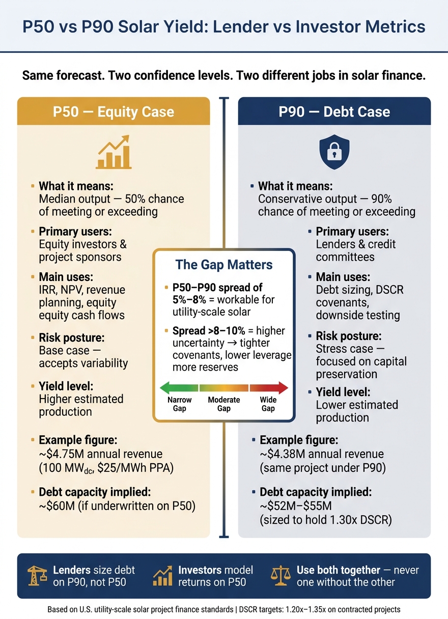
Quick Comparison
| Item | P50 | P90 |
|---|---|---|
| What it means | Median output case | Lower output case with 90% chance of being met or beaten |
| Main user | Equity investors and sponsors | Lenders and credit teams |
| Main use | Return model, IRR, NPV, planning | Debt sizing, DSCR, downside testing |
| Yield level | Higher | Lower |
| Risk view | Base case | Stress case |
| What the gap shows | Forecast uncertainty when compared with P90 | Forecast uncertainty when compared with P50 |
What I like about the piece is that it keeps the message simple: you should not pick one metric and ignore the other. P50 without P90 can make a project look stronger than a lender will accept. And P90 without P50 can miss the return case that equity cares about. The article also ties this back to project review, model control, and keeping finance assumptions lined up from development through close.
So if I were summarizing the full guide for a U.S. solar team, I’d say this: use P50 to judge the upside of the business case, use P90 to test whether the capital stack can hold, and watch the spread between them because that’s where forecast risk shows up fast.
P50 vs P90: Definitions and Core Differences
Before getting into how lenders and investors use these figures, it helps to pin down what each one means. P50 and P90 are not two different models. They are two confidence levels taken from the same forecast distribution. In project finance, the distance between them shows how much downside risk a project may need to handle.
P50 is the median annual energy yield estimate. In about half of modeled years, actual generation is expected to meet or beat this number. Put simply, it is the central production case.
P90 is the more cautious case. In about 9 out of 10 modeled years, actual generation is expected to meet or beat this number. It sits below P50 on purpose. A stricter confidence threshold leads to a lower yield estimate.
How Probability of Exceedance Works
Probability of exceedance measures the chance that actual production will meet or beat a stated yield. If a project has a P90 forecast of 92,000 MWh, that means there is a 90% chance it will generate at least that much in a given year. If the same project has a P50 forecast of 100,000 MWh, there is only a 50% chance of reaching that level or more.
That difference matters. Lenders are not focused on the middle-of-the-road outcome. They want to know whether the project can hold up in a weaker year, after factoring in weather swings, modeling error, and equipment underperformance before any of it happens. That is why lenders size debt from P90, not P50.
P50 vs P90: Side-by-Side Comparison
| Feature | P50 (Median Case) | P90 (Conservative Case) |
|---|---|---|
| Exceedance probability | 50% – equal chance of over or under | 90% – high confidence of meeting or exceeding |
| Position in distribution | Midpoint / median | Lower end / downside |
| Level of conservatism | Less conservative | More conservative |
| Primary use case | Equity return modeling, revenue planning | Debt sizing, downside risk analysis |
| Confidence level | Central expected output | Downside-protected output |
| Relative yield value | Higher estimated production | Lower estimated production |
Both figures come from the same technical base. If the gap between them is large, that points to more uncertainty in the forecast. The cause might be weather variability, weaker resource data, or broader modeling assumptions. In plain English: a wider gap means more forecast uncertainty.[2]
With the definitions in place, the next step is to see how each case shapes financing. Lenders and investors do not use these figures the same way when sizing debt and modeling returns.
How Lenders and Investors Use Each Yield Case
Lenders and equity investors may look at the same yield forecast, but they don’t use it the same way. Lenders size debt off P90. Investors build return cases off P50. That split shapes the bankability model, the debt package, and the rest of the finance stack.
Why Lenders Use P90 for Debt Sizing
Lenders start with the downside case. They take the P90 output and turn it into cash flow using contracted prices, incentives, operating costs, reserves, and taxes. From there, they size debt so DSCR stays above the loan covenant – often 1.20x–1.35x for contracted projects, and higher when merchant exposure is part of the mix.
Here’s what that looks like in practice. On a 100 MWdc project with a 20-year $25/MWh PPA, P50 revenue is about $4.75 million. Under P90, that drops to about $4.38 million. That gap can pull debt capacity down from roughly $60 million to about $52 million–$55 million if the goal is to hold 1.30x DSCR.
That P90-based debt case sets the financing floor for the rest of the model.
Why Investors Model Returns from P50
Equity investors look at P50 as the expected case. They use it to model revenue, cash flow, IRR, and NPV. In U.S. utility-scale solar, sponsors often aim for low-teens equity IRR targets, and those return calculations are usually built on P50 assumptions. In plain English: P50 is the base case for equity returns. [7][8]
That doesn’t mean investors ignore downside risk. They still test P75, P90, and sometimes P99 to see how the project holds up under stress. But when the team talks about expected returns, P50 is usually the number at the center of the conversation. [7][8]
That same P50 case then moves into internal review and equity planning.
Debt Case vs Equity Case: Comparison Table
| Aspect | P50 (Equity Case) | P90 (Debt Case) |
|---|---|---|
| User | Equity investors, sponsors | Lenders, credit committees |
| Use | IRR, NPV, equity cash flows | Debt sizing, DSCR covenants |
| Risk posture | Moderate to high – accepts variability | Low – focused on capital preservation |
| Cash-flow basis | Expected annual revenue | Stressed annual revenue |
| Key outputs | Equity IRR, project IRR, NPV, payback | Debt size, DSCR, reserve requirements |
| Binding only in debt case | Shown for reference | Binding covenant sized on P90 cash flow |
One point matters more than it may seem: equity models should use the P90-approved debt schedule, not a more aggressive leverage case that looks good only on paper. [8] That’s how solar teams keep development assumptions lined up with what lenders will actually support.
Risk, Bankability, and the P50-P90 Gap
Once P50 is assigned to equity and P90 to debt, the next issue is the size of the gap between them. That P50–P90 gap is a plain measure of forecast uncertainty and bankability. A narrow gap usually means the forecast rests on solid support. A wider gap usually points to weaker data, site limits, or shakier modeling assumptions.
What Drives the Gap Between P50 and P90
Several factors can push the gap wider: weather swings, resource-data quality, degradation, soiling, curtailment, and modeling error. Stack those together, and the total spread can go past 10%. Projects with high DC/AC ratios and more complex tracking systems often show a wider spread. Fixed-tilt systems with more conservative DC/AC ratios usually keep the range tighter. Industry guidance says the P50–P90 spread should stay at or below 8%.[9]
What Makes a Yield Forecast Bankable
A bankable yield forecast relies on transparent inputs, defensible methods, and a documented process for building the uncertainty band that lenders and independent engineers can audit. Put simply, if someone reviews the model line by line, they should be able to see how the forecast was built and why the range makes sense.
The table below shows how that gap shapes lender confidence and debt sizing.
Risk Level and Financing Confidence: Comparison Table
| Dimension | P50 | P90 |
|---|---|---|
| Risk | Moderate – expected case with both upside and downside potential | Low – conservative case with built-in downside protection |
| Lender comfort | Low | High – primary basis for lender debt sizing |
| Debt sizing | Maximum potential debt capacity if the expected case were underwritten | Practical bankable debt capacity, lower but credit-aligned |
| Error sensitivity | High – optimistic assumptions directly affect the central estimate | Lower – conservative inputs reduce exposure, though a wide gap still signals residual uncertainty |
For utility-scale projects in the U.S., a P50–P90 gap in the 5% to 8% range usually supports comfortable debt sizing.[9] If that gap starts to widen, lenders often respond by tightening covenants, cutting leverage, or asking for reserves. That’s why solar teams use the spread as a stress test before a project moves into review and financing.
How Solar Firms Apply P50 and P90 in Project Review and Finance Planning
Where Each Metric Fits in the Project Lifecycle
P50 and P90 show up at different points in the project lifecycle, and each one serves a different job.
At origination and early screening, P50 leads the way. Developers use the base-case yield estimate to check, fast, whether a project clears internal hurdle rates and lines up with strategic goals. P50 also helps shape early development budgets.
By the time a project gets to the investment committee, both cases are in play. Teams look at IRR, DSCR, and cash flow coverage side by side under P50 and P90. Then they dig into the gap between the two: How wide is the production spread? Does P90 still cover debt service? Are degradation, availability, soiling, and curtailment assumptions lined up across both runs? After that, financing teams start tightening the model around the downside case.
At financing, P90 usually becomes the debt case, while P50 stays the equity reference. At that point, forecast governance moves to the front of the line.
Pre-close risk checks bring both cases back together for one last validation pass. Teams re-run downside scenarios that pair P90 production with stressed prices and operating costs. They also confirm that degradation and availability assumptions match across both cases and confirm the post-close operating benchmark.
Keeping Forecast Assumptions Aligned Across Finance and Operations
The day-to-day challenge is simple to describe and hard to manage: keeping both cases in sync as a project moves from development into operations. If teams are working out of separate spreadsheets, drift starts to creep in. And once that happens, lenders often recalculate DSCRs.
Firms that handle this well put clear forecast governance in place. That usually means:
- A designated model owner who controls P50/P90 templates
- A standard parameter library for resource inputs and loss assumptions
- A change-control process that requires documented sign-off before any assumption is revised
When those assumptions stay aligned, the finance case remains usable through close.
Shared systems can make that a lot easier. In Blu Banyan‘s SolarSuccess on NetSuite, teams can control P50/P90 templates, route approvals, and sync project, finance, and reporting data in one system.[11]
That keeps project review, diligence, and operating plans tied back to the same set of assumptions.
Conclusion: Using P50 and P90 Together for Better Finance Decisions
When finance and operations are working from the same assumptions using solar business management software, the last piece is deciding how P50 and P90 shape capital decisions.
P50 is used for expected-return modeling. P90 is used for debt sizing and downside testing. Lenders size debt to P90 and want covenant headroom. That split is the whole idea.
Bankability comes down to inputs that can be defended, clear uncertainty analysis, and consistent assumptions across technical and financial models. In plain English, lenders look at the model itself, not just the headline numbers. That link runs from development to finance to operations, and forecast governance is what holds it together.
Used together, P50 and P90 show expected performance and downside risk – the core of bankable solar finance.
FAQs
How is P90 calculated from a solar yield forecast?
A P90 yield estimate uses statistical modeling to pinpoint the level of energy production that has a 90% chance of being exceeded over a set period.
Analysts build this estimate using past solar irradiance data, weather patterns, and site conditions to map out a range of possible results. Compared with P50, P90 relies on more conservative assumptions to account for variability and risk.
When should a project use P75 or P99 instead of just P50 and P90?
Use P75 or P99 when a project needs more certainty than P50 and P90 can offer.
These estimates make sense when investors or lenders want extra protection against production shortfalls. They also fit projects with high-value components or long-term financing, where stricter performance guarantees matter more.
What can developers do to narrow the P50-P90 spread?
Developers can narrow the P50-P90 spread by cutting technical and day-to-day uncertainty with better project data and smoother execution.
A lot of that comes down to getting everyone on the same system. When operations run through one ERP, teams can work from the same project-linked data for equipment, labor, and soft costs instead of piecing things together from scattered tools and spreadsheets.
That matters because cleaner data usually leads to better forecasts. And when teams track milestones automatically, they can spot issues earlier and deal with risk before the spread starts to widen.
